Remember TS? We implicitly assumed that at state $s$, taking action $a$ leads to a single next state $s’$.
Well, life sucks and in the real world, there is a chance you end up in different states for one reason or another.
Determinism is your ability to predict exactly what state you’ll end up in.
Determinism is the level by which an action $a$ taken in state $s$ determines the next state $s’$.
There are three levels of determinism:
Deterministic: Taking action $a$ in state $s$ always
Non-deterministic: Taking action $a$ in state $s$ may lead to one of several possible next states
Stochastic: Taking action $a$ in state $s$ leads to one of several possible next states according to some probability distribution (probability distribution just refers to the odds of ending up in each possible next state)
Why bother? Because the level of determinism affects:
What formalism you can use to model the environment
What algorithms you can use to search/solve the environment
How complex the environment is to reason about
How realistic your model is
As such, what you need to know about each level:
The definition of course
What formalisms are expressive enough to model it
What algorithms can be used to search/solve it
What the outcome of solving it looks like (e.g., plan vs policy)
When/why to use it in your AI problems
Levels of Determinism in a Nutshell
Determinism Level
Definition
Formalism
Algorithms
When/Why to Use
Deterministic
$a$ in $s$ always leads to one $s’$
Transition System (TS)
DFS, BFS, UCS, A*
Simple problems, fully predictable environments
Non-deterministic
$a$ in $s$ may lead to multiple $s’$
Nondeterministic TS (NTS)
AND-OR search, Contingency Planning
Environments with uncertainty but no probabilities
Stochastic
$a$ in $s$ leads to $s’$ with probability $P(s’)$
Markov Decision Processes (MDPs)
Value Iteration, Policy Iteration, Q-learning
Real-world problems with uncertainty and probabilistic outcomes
** Final Exam Checklist **
I know what determinism is and why we study it (other than to be able to answer final exam questions).
I know the three levels of determinism and their definitions.
I am able to recite the table above (formalism, algorithms, when/why to use).
I know how transitions are modeled in deterministic environments (i.e., I know what a deterministic transition function is, and what its signature looks like).
I know which formalisms can model deterministic environments (its just TS in our course).
I know what algorithms can be used to search/solve deterministic environments (DFS, BFS, UCS, A*).
I know what the outcome of solving a deterministic environment looks like (a plan).
I know what a plan is (its a sequence of actions), what it is not (its not a function), and how to execute it (just execute the actions in order).
Kinda weird having the final exam checklist longer than the actual section, right?
In non-deterministic environments, taking action $a$ in state $s$ may lead to one of several possible next states. Implications, you say?
3.1. Modeling - NDTS
Our beloved transition function $T : S \times A \to S$ no longer works,
Which means TS can’t model non-deterministic environments.
Which means we need a new formalism that can handle multiple possible outcomes.
How about we have the same transition function, BUT, instead of mapping to a single next state, it maps to a set of possible next states? What a brilliant idea.
Nondeterministic Transition Function: $T : S \times A \to 2^S$ (the power set of S, aka the set of all subsets of S).
3.1.1. Intermission: What is $2^S$?
Q: What is $2^S$?
A: The power set of S, aka the set of all subsets of S.
Q: Wot?
A: Let’s say the robot moves between two rooms (two grid cells), rooms 1 and 2.
So the state space is $S = \lbrace s_1, s_2 \rbrace$.
So the powerset is $2^S = \lbrace \emptyset, \lbrace s_1 \rbrace, \lbrace s_2 \rbrace, \lbrace s_1, s_2 \rbrace \rbrace $.
Q: $\emptyset$-what?
A: The empty set, aka the set with no elements, also written as { }.
3.1.2. Nondeterministic Transition System (NDTS)
A Nondeterministic Transition System (NDTS) is a tuple $(S, A, T)$ where:
$T : S \times A \to 2^S$ is the nondeterministic transition function
This is modeled using a nondeterministic transition function: $T(s, a) \subseteq S$
This means that $T(s, a)$ is a set of possible next states.
We informally discussed AND-OR search and Contingency Planning in lecture.
What you need to know for the final exam:
AND-OR search and Contingency Planning are algorithms that can be used to search/solve non-deterministic environments.
The outcome of solving a non-deterministic environment is a contingency plan.
A contingency plan is a tree of actions and outcomes.
To execute a contingency plan, you follow the path based on actual outcomes.
For example, if you take action $a$ in state $s$ and end up in state $s’$, you follow the branch of the contingency plan corresponding to $s’$.
So, think of it as a bundle of plans, one for each possible outcome.
3.3. Solving Outcomes - Contingency Plan *
The outcome of solving a non-deterministic environment is a contingency plan.
Again… a contingency plan is a tree of actions and outcomes.
Forma..
* Q: WAIT A MINUTE… We never covered this in lecture, did we?
A: Correct, we only covered the concepts themselves through examples and discussions. But we never mentioned AND-OR search or Contingency Planning or whatever that is.
Q: Why?
A: Because, in practice, you will never use AND-OR search. The algorithm itself is not like a novel thing that we could learn from or something. I don’t even know why this exists. Actually, I do know – it is only used in teaching as a transition (moving between topics, not our transition function) from deterministic search to stochastic search. But in practice, this is never used. So, moving on. Rant ends.
HOWEVER… We covered important insights through examples and discussions
Some of those important insights:
a) When searching/solving non-deterministic environments, you consider THE WORST-CASE outcome.
Meaning: you have 11 cards: numbers from 1 to 10 and one Queen (all hidden from you, you don’t know which is which). If you choose your next action to be “pick a card”, you have one of 11 outcomes:
Ending up with any of the 10 numbered cards earns you $1 times the card number
Ending up with the Queen takes away $2 from you (not again…)
Your goal is to maximize your minimum guaranteed reward (the worst-case).
You can play or pass.
If you choose to play (take that action that has 11 possible outcomes), you are making a huge mistake.
Why? Because in the worst-case, you lose $2, even though you logically think that it is 10 times more likely that you get a numbered card than the Queen.
Non-deterministic search is a pessimistic one. The worst will always happen. Murphy’s law and what not.
b) If any of the outcomes leads to failure/hazard state, then the whole action is considered to lead to failure/hazard.
Again, worst-case thinking.
c) The goal is usually to reach a goal state with absolute certainty.
Remember: we didn’t need to worry about possible outcomes when we were in deterministic environments using TS along with DFS. The good old days.
3__** Final Exam Checklist **__
I know how transitions are modeled in non-deterministic environments (i.e., I know what a non-deterministic transition function is, and what its signature looks like).
I know which formalisms can model non-deterministic environments (Nondeterministic Transition Systems).
I know what algorithms can be used to search/solve non-deterministic environments (AND-OR search, Contingency Planning).
I have no clue how those algorithms work, and that’s fine because I don’t need to know that for the final exam (or for anything for that matter).
But I know that solving non-deterministic environments entails considering the worst-case outcomes.
I know what the outcome of solving a non-deterministic environment looks like (a contingency plan) and that it is a tree of actions and outcomes (a bundle of plans).
Slogan: One State ~ One Action ~ Multiple Probabilistic Outcomes
In stochastic environments, taking action $a$ in state $s$ leads to one of several possible next states, each with some probability.
4.0. Probability Theory
If you are familiar with basic probability theory, you can skip this section. Otherwise, brace for impact.
To understand probabilities, you need to get very, very comfortable with a few key concepts. You need to be able to read and understand the following notation:
Conditional Probability Notation
\[\Huge P(s' \mid s, a) = p_{ss'}^{a}\]
*The **probability** of transitioning to $s'$ **given that** we are in $s$ and take action $a$ is $p_{ss'}^{a}$.*
Random Event: An outcome that cannot be predicted with certainty. In this course:
Transitioning to a particular state $s’$ is the random event.
The transition $s \xrightarrow{a} s’$ is a random event (because taking action $a$ in state $s$ can lead to multiple possible next states).
Probability: A number between 0 and 1 that indicates how likely an event is to occur.
$p_{ss’}^{a}$: the probability of transitioning to $s’$ when taking action $a$ in state $s$, a number between 0 and 1.
$p_{ss’}^{a} = 0.4$: the probability of transitioning to $s’$ when taking action $a$ in state $s$ is 40% likely to happen.
$p_{ss’}^{a} = 1$: it means that $\;s \xrightarrow{a} s’ \;$ is a deterministic transition (100% chance of landing in $s’$).
Probability Function: A function $P: \text{event-space} \to [0,1]$ that assigns probabilities to events.
$P(s’)$: the probability of transitioning to $s’$ (from anywhere).
$P(X=3)$: the probability that random variable $X$ takes the value 3.
Conditional Probability: The probability of an event occurring given that another event has occurred… What?
Let’s say you have four cards:
\[\Large [3♠], [3♠], [5♠], [8♥]\]
Cards are shuffled and hidden from you.
Suppose that you pick a card (randomly), and this card turns out to be a [5♠]. Picking [5♠] is called a random event.
How likely that this (random event) happens? \(P(\text{picking a 5}) = \frac{1}{4} = 0.25\)
Let’s refer to picking the first card as $X$, and to that event (picking a 5) as $X_1=5$. Then, we can write: \(P(X_1=5) = 0.25\)
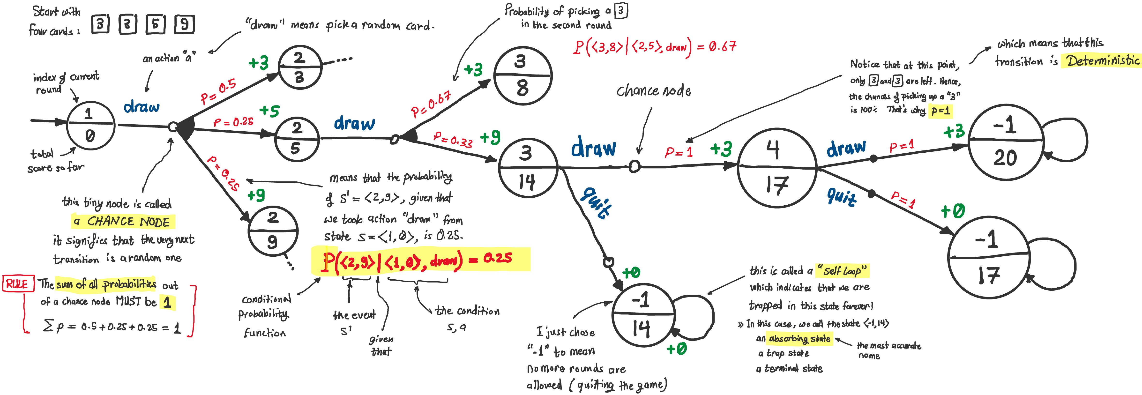
Now, let’s refer to picking a second card as $X_2$. What is the probability of picking a 3 in the second round ($X_2=3$), given that you already picked a 5 ($X_1=5$)? This is called conditional probability, and is written as:
\(P(X_2=3 \mid X_1=5) = \frac{2}{3} \approx 0.67\)
If you are still confused, that’s okay. Things will clear up a bit as we resume our discussion on stochastic environments in this very next section.
4.1. Modeling - MDPs
The formalism that models stochastic environments is called Markov Decision Processes (MDPs).
A Markov Decision Process (MDP) is a tuple:
\[\Huge \mathcal{M} = (S, A, T, R, \gamma)\]
where:
$S$ and $A$ are the same as before in TS (state space and action space).
$T : S \times A \times S \to [0,1]$ is the stochastic transition function (or transition model, or probabilistic transition function, or transition function, … lots of names out there).
Remember $T(s, a) = s’$ in TS? It’s not useful here because we now need a different function that can express multiple possible next states with probabilities.
$T(s,a,s’)$ is the probability of transitioning to state $s’$ when taking action $a$ in state $s$.
Be careful: $T(s,a)$ and $T(s,a,s’)$ are different functions!
$R : S \times A \times S \to \mathbb{R}$ is the reward function.
$R(s,a,s’)$ is the immediate reward received after transitioning from state $s$ to state $s’$ via action $a$.
Note: sometimes, the reward function is defined as $R : S \to \mathbb{R}$, where $R(s)$ is the reward for being in state $s$. Both definitions are valid; it depends on the specific MDP formulation.
I can only imagine how confusing this must be right now. That’s why I started the lectures with the card game examples so you can see the transitions, probabilities, and rewards in action first, before throwing formal definitions at ya.
In any case, let’s look at the two key changes here compared to TS:
4.1.1. Stochastic Transition Function
It’s just a way for expressing that there can be multiple possible next states (outcomes), and that we can quantify the probability of each (i.e., how likely each outcome is to happen).
Warning / Attention / Achtung / Ojo / Attenzione / Atenção / تنبيه / 注意 / 注意 / 주의 / सावधान / Внимание / Wee-Woo
All those three functions are called “transition functions”, but they are different functions!
Signature
Notation
Output
Determinism Level
Appears in
$T: S \times A \rightarrow S$
$T(s,a) = s’$
$s’ \in S $
Deterministic
TS
$T: S \times A \rightarrow 2^S$
$T(s,a) = \lbrace s’_1, s’_2, …\rbrace$
$ S’ \subseteq S $
Nondeterministic
NDTS
$T: S \times A \times S \rightarrow [0,1]$
$T(s,a,s’) = p_{ss’}^a$
$p \in [0,1]$
Stochastic
MDPs, POMDPs
Proof they are different:
All three functions have different signatures. Hence, they are different functions, which completes the proof.
4.1.2. Reward Function
It is just a way to express that some states or transitions are better / worse than others.
\[\Huge R : S \times A \times S \to \mathbb{R}\]
$R(s,a,s’)$ is the immediate reward received after transitioning from state $s$ to state $s’$ via action $a$.
Personally, I call this XP or “experience points” because it sounds cooler and more meaningfull than transition reward.
Warning / Attention / Achtung / Ojo / Attenzione / Atenção / تنبيه / 注意 / 注意 / 주의 / सावधान / Внимание / Wee-Woo
You will see in literature three types of reward functions:
Signature
Notation
Output
Significance (When to Use)
Formalism Where They Appear
$R: S \rightarrow \mathbb{R}$
$R(s)$
$r_s \in \mathbb{R}$
Rewards being in a state, independent of how you got there or what you do next
MDPs, goal-based planning, grid worlds with terminal rewards
$R: S \times A \rightarrow \mathbb{R}$
$R(s,a)$
$r_s^a \in \mathbb{R}$
Rewards state-action pairs, capturing cost/benefit of taking specific actions in specific states
MDPs, Q-learning, action costs (e.g., moving vs. staying), resource consumption
$R: S \times A \times S \rightarrow \mathbb{R}$
$R(s,a,s’)$
$r_{ss’}^a \in \mathbb{R}$
Rewards transitions, outcome-dependent rewards
MDPs, transition-based penalties, full generality
Note: In the final exam, you will be explicitly told which of the three reward function types to use in a given question.
But, why do we need rewards in the first place???
Intuitively, we want to be able to express that some outcomes are more desirable than others.
For example: in card games from lecture, getting a high-value card (more money) is better than getting a low-value card (less money). You win in both cases, but one is better than the other.
Real reason: To guide the agent toward optimal behavior by assigning rewards to states and transitions. In other words, it helps the search algorithm figure out which paths are better than others.
4.1.3. Discount Factor
Ehh, don’t worry about it for now.
4.1.4. Example MDP: Four-Card Game
In this game:
the dealer shuffles four cards: [3♠], [3♠], [5♠], [9♥].
You can either “draw” (pick) a card or “quit” (leave with current score).
You start round 1 with score 0. So, your initial state is $s_0 = \langle 1, 0 \rangle$.
You can also keep drawing cards until you have all four cards.
Let’s ignore the agent’s goal for now.
And yes, it is a meaningless game. You will play it now anyway because you will play a similar on in the final exam.
Carefully study the following state transition diagram of an MDP model for this four-card game (only part of the diagram is shown)
Some of the things to pay attention to:
The way we graphically represent probabilistic transitions:
States are represented as circles or nodes (sometimnes as capsules or rectangles for aesthetics).
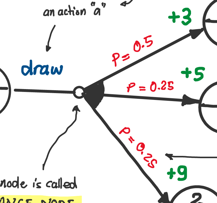
The first segment of the arrow (from state to small circle) is labeled with the name of the action taken.
The small circle is called a “chance node”. Semantically, it represents the point in time where you decided the action to take, but the outcome is still unknown.
The second segment of the arrow (from small circle to next state) is labeled with the probability of that outcome happening.
The tails of those segments meet at the chance node, with an arc (the black sector) connecting them together to indicate that they are part of the same action, but branching out to different possible outcomes.
The sum of probabilities of all outgoing transitions from a chance node must equal 1.
When there is only one possible outcome, we sometimes omit the chance node and probability label for simplicity. Also, in that case, the transition is deterministic.
Sometimes we show the reward associated with a transition as a label on the arrow head (+3, +5, and +9 in this example).
On a side note. You will see this state transition diagram referred to as “state transition graph” or “state transition model” or “state transition diagram” or “MDP graph” or “MDP model” or “MDP diagram” or whatever. They all refer to the same thing. The “state transition diagram” is the most accurate. The “MDP model”, or the “MDP” for short, is the most commonly used. So from now on, we will refer to it as the “MDP”.
Now that we know how to model stochastic environments (hint: we use MDPs), the next question is: how do we search/solve them?
Actually, before that, what does it even meant to “solve” an MDP?
Recall back in the old days of TS and DFS, solving meant finding a plan (sequence of actions). As we showed in the lecture, that doesn’t work here because, you don’t know which state you will end up in along the way. Taking actions blindly without knowing the actual outcomes is like trying to find a parking in APS with a blindfold.
The solution is to adapt your actions based on the actual outcome, i.e., based on what state you actually end up in after each action. We call such a solution a policy.
4.2.1. Policy
\[\Huge \pi: S \to A\]
A policy $\pi$ is a function that maps each state $s \in S$ to an action $a \in A$.
In other words, a policy tells the agent what action to take in each state.
4.2.2. Solving MDPs - DIWhy Method
I like to start with examples. Let’s start with the simplest example possible. Be careful though, as we go, we will add more complexity to the same example, so make you pay attention to what applies to which version of the example. In general:
R: the robot
G: the goal
$\langle x, y \rangle$: the state, which is only the robot’s position on the grid
$R(s, a, s_4) = +10 \quad$ (anything that leads to goal is rewarded 10 points)
$\forall s’ \neq s_4: R(s, a, s’) = 0 \quad$ (anything that doesn’t lead to goal is rewarded nothing)
Discount factor: $\gamma = 1$ (no discounting… because we don’t know what discounting is yet.)
Goal:
Find the optimal policy $\pi^*$ that maximizes expected cumulative reward.
Since we have no clue what that means yet, let’s just say we want to
find the best action to take in each state so we end up with the highest score possible.
Method: We’ll use Value Iteration - repeatedly apply the Bellman equation until values converge. We don’t know what any of that means, and that’s okay, remeber this:
Best state is the one that has highest potential to get you the most points.
Best action at a given state is the one that gives this state the highest potential to get you the most points.
The highest potential of a state is called its value, denoted $V(s)$.
Iteration 0: Create an empty state-action-value table:
State
$\; N \;$
$\; E \;$
$\; \tau \;$
$V(s)$
Optimal Action
$s_1 = \langle 1, 1 \rangle$
0
0
0
0
?
$s_2 = \langle 2, 1 \rangle$
0
0
0
0
?
$s_3 = \langle 1, 2 \rangle$
0
0
0
0
?
$s_4 = \langle 2, 2 \rangle$
0
0
0
0
?
This simply means that, before any transitions happen, you’ve got no points.
Iteration 1: Your total value = what you already have + what you expect to get from taking action $a$ in state $s$.
State
$\; N \;$
$\; E \;$
$\; \tau \;$
$V(s)$
Optimal Action
$s_1 = \langle 1, 1 \rangle$
0
0
0
0
?
$s_2 = \langle 2, 1 \rangle$
0+10
0
0
10
E
$s_3 = \langle 1, 2 \rangle$
0
0+10
0
10
N
$s_4 = \langle 2, 2 \rangle$
0
0
0
0
?
Row 2: Moving east leads to goal, so you get 10 points. The best action is E. The best action will get you 10 points, so $V(s_2) = 10$ (so far).
Row 3: Moving north leads to goal, so you get 10 points. The best action is N. The best action will get you 10 points, so $V(s_3) = 10$ (so far).
Iteration 2: Repeat the process
State
$\; N \;$
$\; E \;$
$\; \tau \;$
$V(s)$
Optimal Action
$s_1 = \langle 1, 1 \rangle$
0+10
0+10
0
10
E or N
$s_2 = \langle 2, 1 \rangle$
10
0
0
10
E
$s_3 = \langle 1, 2 \rangle$
0
10
0
10
N
$s_4 = \langle 2, 2 \rangle$
0
0
0
0
?
Iteration 3: Repeat the process.
State
$\; N \;$
$\; E \;$
$\; \tau \;$
$V(s)$
Optimal Action
$s_1 = \langle 1, 1 \rangle$
10
10
0
10
N or E
$s_2 = \langle 2, 1 \rangle$
10
0
0
10
N
$s_3 = \langle 1, 2 \rangle$
0
10
0
10
E
$s_4 = \langle 2, 2 \rangle$
0
0
0
0
?
Hmmm it looks like nothing has changed. So we can stop here.
Final Policy: $\pi^*$ is defined as follows:
State
Optimal Action
$s_1 = \langle 1, 1 \rangle$
N or E
$s_2 = \langle 2, 1 \rangle$
N
$s_3 = \langle 1, 2 \rangle$
E
$s_4 = \langle 2, 2 \rangle$
?
So, what does that mean for $s_4$? You have one of two choices:
You can say “there is no optimal action in the goal state because the game ends there”.
In that case, $\pi(s_4)$ is undefined, and $\pi$ is a partial function.
Interpretation: once you reach the goal, the policy’s job is done and there is nothing else for it to tell you.
Or you can say “the optimal action in the goal state is to do nothing ($\tau$) because you have already won”.
In that case, $\pi(s_4) = \tau$, and $\pi$ is a total function.
Interpretation: once you reach the goal, the policy tells you to stay put and do nothing. This is your life now.
[b] Grid World - 2x2 - Slippery Actions
What changed:
Transitions: Stochastic
Intended action succeeds 80% of the time
Slip perpendicular 10% each direction
$\tau$ always works (100%)
Iteration 0:
State
$\; E \;$
$\; N \;$
$\; \tau \;$
$V(s)$
Optimal Action
$s_1 = \langle 1, 1 \rangle$
0
0
0
0
?
$s_2 = \langle 2, 1 \rangle$
0
0
0
0
?
$s_3 = \langle 1, 2 \rangle$
0
0
0
0
?
$s_4 = \langle 2, 2 \rangle$
0
0
0
0
?
Iteration 1:
State
$\; E \;$
$\; N \;$
$\; \tau \;$
$V(s)$
Optimal Action
$s_1$
0
0
0
0
?
$s_2$
0.8(0) + 0.1(10) + 0.1(0) = 1
0.8(10) + 0.1(0) + 0.1(0) = 8
0
8
N
$s_3$
0.8(10) + 0.1(0) + 0.1(0) = 8
0.8(0) + 0.1(10) + 0.1(0) = 1
0
8
E
$s_4$
0
0
0
0
?
Iteration 2:
State
$\; E \;$
$\; N \;$
$\; \tau \;$
$V(s)$
Optimal Action
$s_1$
0.8(8) + 0.1(8) + 0.1(0) = 7.2
0.8(8) + 0.1(8) + 0.1(0) = 7.2
0
7.2
E or N
$s_2$
1
0.8(10) + 0.1(0) + 0.1(7.2) = 8.72
0
8.72
N
$s_3$
0.8(10) + 0.1(0) + 0.1(7.2) = 8.72
1
0
8.72
E
$s_4$
0
0
0
0
?
Iteration 3:
State
$\; E \;$
$\; N \;$
$\; \tau \;$
$V(s)$
Optimal Action
$s_1$
0.8(8.72) + 0.1(8.72) + 0.1(0) = 7.85
0.8(8.72) + 0.1(8.72) + 0.1(0) = 7.85
0
7.85
E or N
$s_2$
1
0.8(10) + 0.1(0) + 0.1(7.85) = 8.79
0
8.79
N
$s_3$
0.8(10) + 0.1(0) + 0.1(7.85) = 8.79
1
0
8.79
E
$s_4$
0
0
0
0
?
Values converge after several more iterations. Actually, you can write the table using a formula:
State
$\; E \;$
$\; N \;$
$\; \tau \;$
$V(s)$
Optimal Action
$s_1$
$0.8V(s_2) + 0.1V(s_3) + 0.1(0)$
$0.8V(s_3) + 0.1V(s_2) + 0.1(0)$
0
$V(s_1)$
E or N
$s_2$
$0.8(0) + 0.1(10) + 0.1V(s_1)$
$0.8(10) + 0.1(0) + 0.1V(s_1)$
0
$V(s_2)$
N
$s_3$
$0.8(10) + 0.1(0) + 0.1V(s_1)$
$0.8(0) + 0.1(10) + 0.1V(s_1)$
0
$V(s_3)$
E
$s_4$
0
0
0
0
?
Final Policy:
Same as variant [a], but values are lower due to uncertainty.