
Back to EECS 31L Index
EECS 31L • Study Notes • Delay Control
Mahmoud Elfar • Spring 2026 • v0.1
v0.1: Initial version
Table of Contents
🕹️ Playgrounds in this note:
See: IEEE 1800-2017, 9.4 Procedural timing controls, pg. 215
Most statements we have seen so far are assignment statements, whether continuous (assign) or procedural (= or <= inside always/initial blocks). The execution of an assignment statement is done in two stages:
What: Delay control here is concerned with controlling the timing of statement execution (evaluation, assignment, or both) in simulation. Delaying the execution of a statement or part of it is controlled by one of two operators:
# for time delays (this note)@ for event delays (future note)This note focuses on the first.
Why: So, why do we need time delays in Verilog in the first place? Two main reasons:
Eitherway, the # operator has no synthesis semantics. It is purely a simulation construct. When you are happy with your design and decide to load it onto an FPGA or send it for fabrication, all # operators disappear.
So, before we proceed, two things to establish upfront:
# is a simulation-only construct. Synthesis tools ignore it entirely. It has no effect on the hardware that gets built.# appears almost exclusively in testbenches. Unless you are studying propagation delays or glitches, you should not write # inside a design module.What we will cover in the rest of this note:
There are two types of time delays in Verilog:
See: IEEE 1800-2017, 9.4.1 Delay control, pg. 216
Syntax:
#<delay>;             // PB; stand-alone delay: just wait
#<delay> a = b;       // PB; wait, then assign
#<delay> a <= b;      // PB; wait, then non-blocking assign
Semantics:
<delay> time units.Example: Those two blocks are equivalent. In both cases, the simulation time advances by 10 units before the evaluation and assignment of the statement a = 1 occurs. In other words: the statement #10 a = 1; is equivalent to the two statements #10; a = 1;.
reg a = 0;
// Block 1
initial begin
  #10 a = 1;
end
// Block 2
initial begin
  #10;
  a = 1;
end
Example: With blocking assignments, the delays are cumulative. Each # adds to the simulation time of the previous statement.
initial begin
  a = 0; b = 0;     // at time 0: set both to 0
  #10 a = 1;        // at time 10: set a to 1
  #10 b = 1;        // at time 20: set b to 1
  #10 $finish;      // at time 30: end simulation
end
Example: With non-blocking assignments, the delays are also cumulative. Just like with blocking assignments, each # adds to the simulation time of the previous statement. The non-blocking assignment operator does not cause delays to restart from t=0.
initial begin
  a = 0; b = 0;     // at time 0: set both to 0
  #10 a <= 1;       // at time 10: set a to 1
  #10 b <= 1;       // at time 20: set b to 1
  #10 $finish;      // at time 30: end simulation
end
Note that each #10 is relative to when the previous statement finished, not relative to time 0. The delays accumulate.
Example:
This playground demonstrates that inter-assignment delays are cumulative regardless of whether blocking or non-blocking assignments are used.
See: IEEE 1800-2017, 9.4.5 Intra-assignment timing controls, pg. 222
An intra-assignment delay places # inside the assignment, between the = or <= and the RHS expression. The RHS is evaluated immediately, but the assignment to the LHS is deferred by the specified number of time units. The word “intra” here means the delay sits within the assignment itself – between evaluating the RHS and writing it to the LHS.
Syntax:
a = #<delay> b;   // evaluate b now, assign to a after <delay> time units
a <= #<delay> b;  // evaluate b now, assign to a after <delay> time units (non-blocking)
Semantics:
The key distinction: with an intra-assignment delay, the RHS is frozen at the moment the statement is reached, and the process continues executing subsequent statements while the write is pending.
Example:
initial begin
  a = 0; b = 1;     // at time 0: set a to 0, b to 1
  a = #10 1;        // at time 0: evaluate RHS (1), schedule a = 1 at time 10
  b = 0;            // at time 0: set b to 0 immediately
  b = #20 1;       // at 0: evaluate RHS (1), schedule b = 1 at time 20
  #30 $finish;      // at time 30: end simulation
end
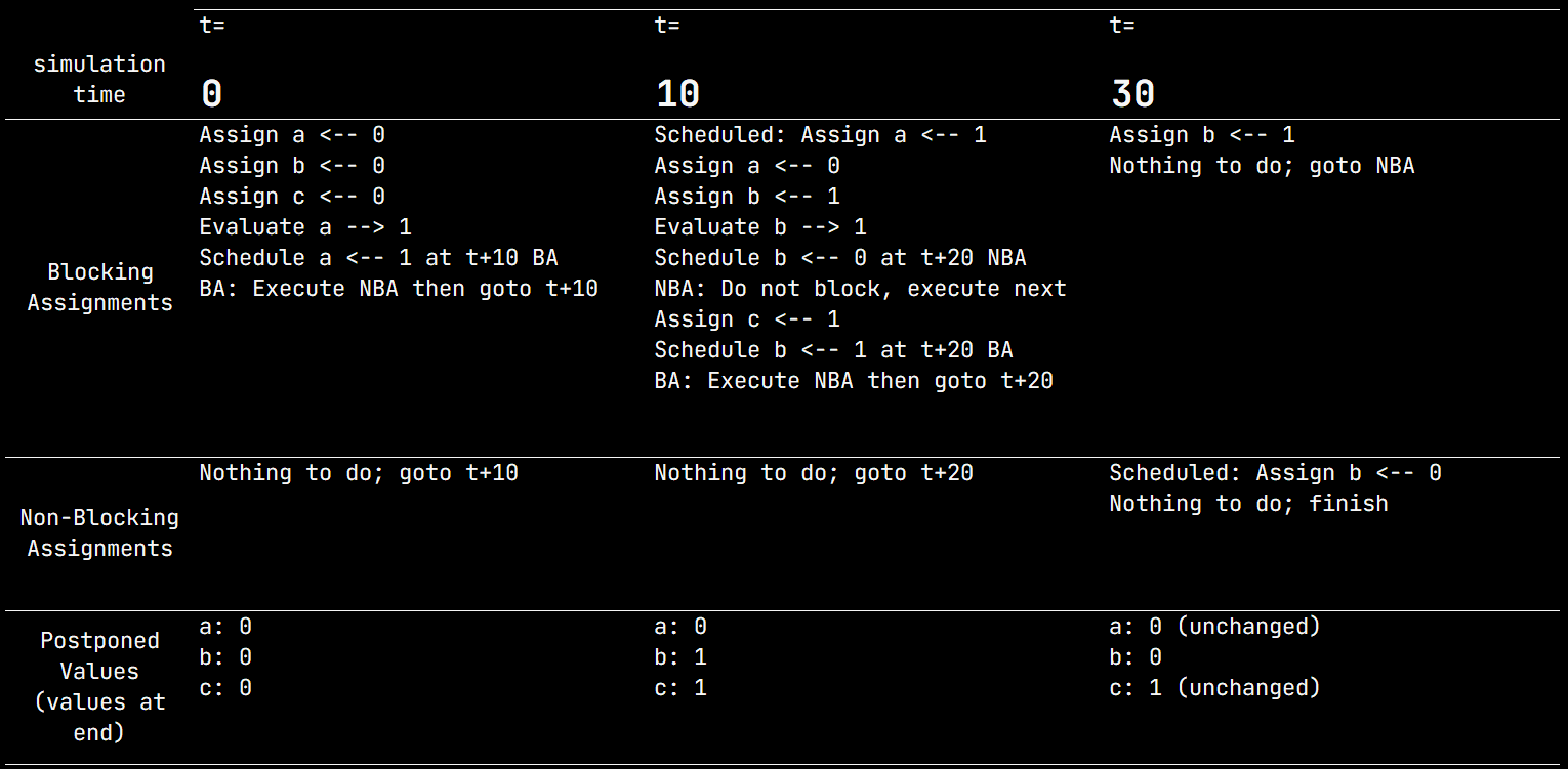
Example:
Unnecessarily complicated, but demonstrates how scheduling works with intra-assignment delays and the order of execution of statements in the same block.
`timescale 1ns / 1ps
`define SIM_TIME 40
module tb_delays_bs_vs_nbs;
  // Initialize all signals to 0 at time 0
  reg a, b, c;
  initial begin
    a = 0; b = 0; c = 0; // t=0: a=0, b=0
    a = #10 1;           // t=0: evaluate RHS (1), jump to t+10, a=1
    a = 0;               // t=10: a=0, immediately override previous assignment
    b = 1;               // t=10: b=1
    b <= #20 0;          // t=10: evaluate RHS (0), do not block execution
    c = 1;               // t=10: c=1
    #20 b = 1;           // t=30: b=1 (BA)
                         // t=30: b=0 (NBA)
  end
  // Dunmp signals for waveform viewing
  initial begin
    $dumpfile("dump.vcd"); $dumpvars;
    #`SIM_TIME $finish;
  end
endmodule
As we stated before, # is ignored by synthesis tools. This means:
#5 a = b or a = b.assign #d y = a & b;.Syntax:
// Placed at the top of a Verilog file, before any module definitions
`timescale <time_unit> / <time_precision>
Semantics:
time_unit specifies the base unit of time for all # delays in the filetime_precision specifies the resolution of time in the simulation, i.e., the smallest time step that can be represented. Delays are rounded to the nearest multiple of the time precision.time_unit and time_precision are specified as a number followed by a time suffix (e.g., 1ns, 100ps, 1us).Example:
`timescale 1ns/1ps
#1 means 1 ns#10 means 10 ns#0.5 means 500 ps (the precision allows fractional units)The time unit applies to all # delays in the file. The time precision determines the smallest representable time step. Fractional delays are rounded to the nearest precision unit.
Clock generation:
The standard pattern uses forever with an inter-assignment delay to toggle the clock every half-period.
`timescale 1ns/1ps

initial begin
  clk = 0;
  forever #5 clk = ~clk;   // 10 ns period, 50% duty cycle
end
Reset pulse:
Assert reset at time 0, release it after a fixed interval.
initial begin
  rst_n = 0;    // assert reset (active low) at time 0
  #20 rst_n = 1; // release reset after 20 time units
end
Stimulus sequencing:
Apply a series of inputs with fixed delays between each.
initial begin
  a = 0; b = 0;
  #10 a = 1;
  #10 b = 1;
  #10 a = 0;
  #10 b = 0;
  #10 $finish;
end
Combining clock and stimulus:
In a real testbench you typically run both concurrently using parallel initial blocks. The two initial blocks run concurrently. The clock generator runs independently of the stimulus block.
`timescale 1ns/1ps
module tb;
  reg clk, rst_n, a, b;
  // Clock generation
  initial begin
    clk = 0;
    forever #5 clk = ~clk;
  end
  // Stimulus
  initial begin
    rst_n = 0; a = 0; b = 0;
    #20 rst_n = 1;
    #10 a = 1;
    #10 b = 1;
    #30 $finish;
  end
endmodule